(Almost) every technique is a linear model
BIOL2022 - L02c
The University of Sydney
Learning objectives
The ideas in this lecture are a bit more abstract than the previous lectures, but they are important to understand as they will help you to:
You should read through this lecture at your own time as it will make your experiments a bit easier to design, assess and interpret.
The general linear model (GLM)
A general (mathematical) framework for expressing relationships between variables.
The basic idea
We are trying to fit a line (or a curve) to the data that best explains the relationship between the variables, essentially a simple equation many of you will be familiar with:
\[y = c + mx\]
where \(c\) is the intercept and \(m\) is the slope of the line.
Compare this to the general linear model: \[y = \beta_0 + \beta_1 x + \epsilon\]
\[y = \beta_0 + \beta_1 x + \epsilon\]
or simply (for your benefit):
\[y \sim x\]
The equation to rule them all, where
- \(y\) is the response variable, or the variable we are trying to predict or explain.
- \(x\) is a predictor variable that can be anything, continuous, categorical, binary, ordinal, etc.
- \(\beta_i\), where \(i\) is an integer, are the coefficients/estimates that quantify the relationship between \(y\) and \(x\).
- \(\epsilon\) is the error term, which captures the variability in \(y\) that is not explained by \(x\).
In general, most common statistical tests can be expressed as a GLM like above.
\[y = \beta_0 + \beta_1 x + \epsilon\]
Why does it matter?
- Under the GLM, the statistical test is identified based on the variables supplied to the model. This follows a model-centric approach:
- If the predictor variable (\(x\)) is binary, we are performing a GLM equivalent to a t-test and the slope is the difference in conditional means.
- If the predictor variable (\(x\)) is categorical, we are performing a GLM equivalent to ANOVA, and the slope represents the difference in means between the categories.
- If the predictor variable (\(x\)) is continuous, we are performing a GLM equivalent to regression. The slope becomes the difference in expected values for a pair of points that differ in \(x\) by one unit.
- For one unit change in \(x\), the expected change in \(y\) is \(\beta_1\).
- The GLM takes care of the “statistical test” for you and you do not need to know what the equivalent test is (although it helps).
How we can use it
- Model the relationship between the response variable and the predictor/explanatory variable(s) as a simple function.
\[response \sim explanation\]
Also read as (recall the previous lecture):
- response is explained by the explanation
- response is a function of the explanation
- response is influenced by the explanation
- …
How we can use it
- Model the relationship between the response variable and the predictor/explanatory variable(s) as a simple function.
\[response \sim explanation\]
- Define the structure of the variables in the model, which can be continuous, categorical, binary, etc., something we can decide if we are the ones designing the study.
\[ (continuous) \sim (continuous) \]
\[ (continuous) \sim (categorical) \]
\[ (binary) \sim (continuous) \]
How we can use it
- Model the relationship between the response variable and the predictor/explanatory variable(s) as a simple function.
\[response \sim explanation\]
- Define the structure of the variables in the model, which can be continuous, categorical, binary, etc., something we can decide if we are the ones designing the study.
\[ (continuous) \sim (categorical) \]
- Fit the model to the data based on the data types, and start work out if the model is a good fit.
\[ response = \beta_0 + \beta_1 \times explanation + \epsilon \]
How we can use it
\[response \sim explanation\]
\[ (continuous) \sim (categorical) \]
\[ response = \beta_0 + \beta_1 \times explanation + \epsilon \]
In most statistical software (including R and Jamovi) you only need to specify the model formula (the first part) and the software will take care of the rest to produce the statistical output (the third part).
Your job is to determine if the model is a good fit, and interpret the results.
A good fit?
Checking assumptions: many ways
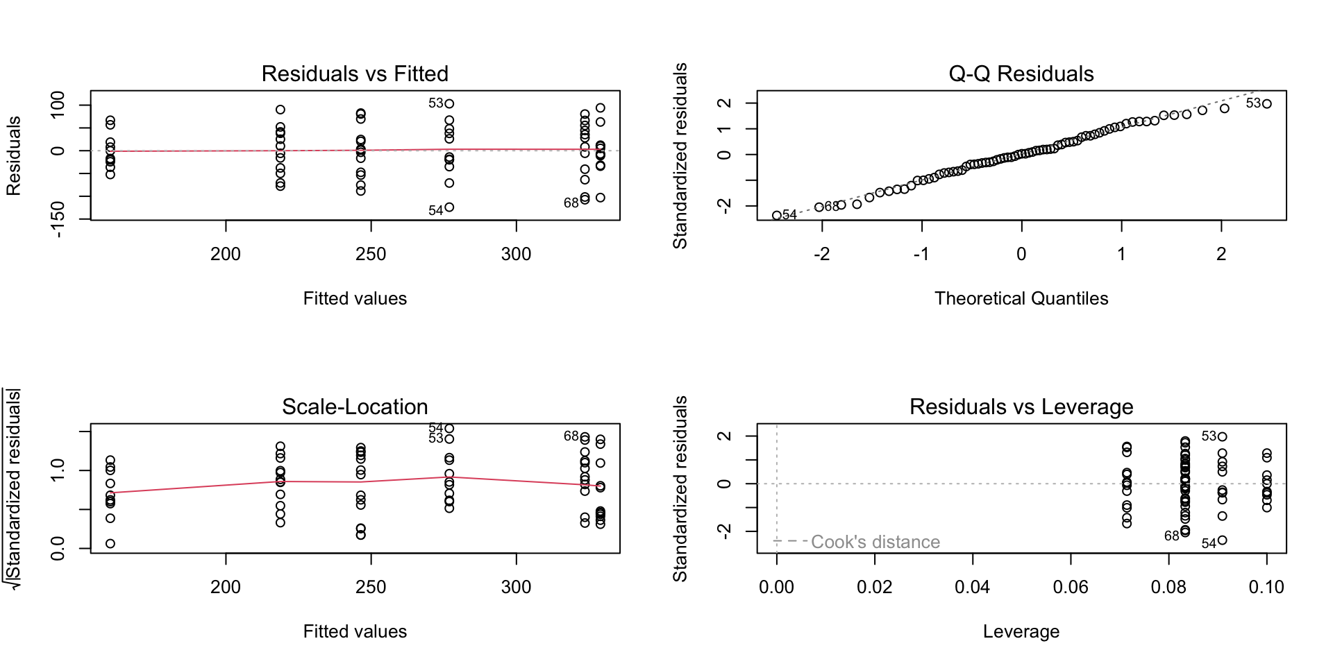
In previous studies, you may have checked assumptions in different ways depending on the statistical test:
- For a t-test, you may have checked for normality by plotting the data and looking for a bell-shaped curve. Equal variances you may have used the F-test or Levene’s test.
- For ANOVA, you may have checked for homogeneity of variance using Levene’s test or Bartlett’s test.
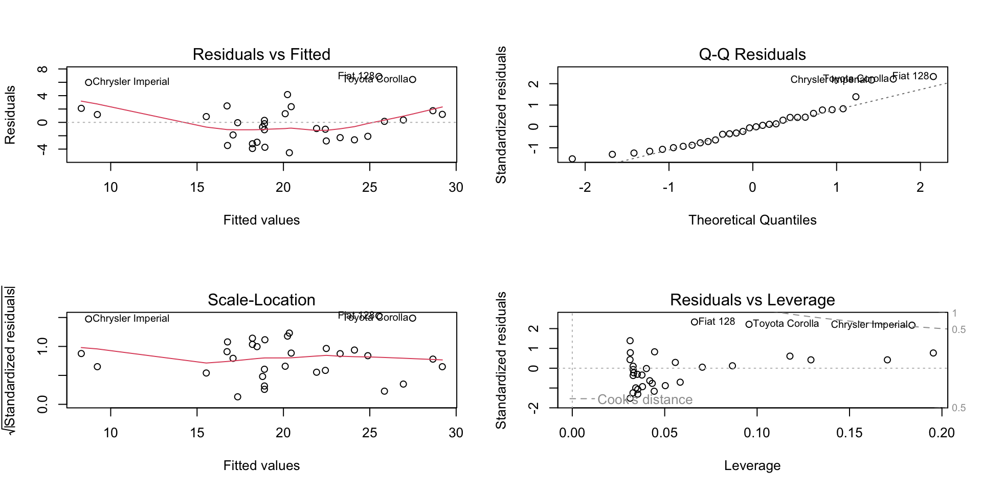
- For regression, you looked at the residuals to check for homoscedasticity and normality.
Checking assumptions: the GLM way
A GLM provides a framework for checking model assumptions using residuals to assess any of:
- Homoscedasticity and Linearity: Are the residuals spread evenly across the range of the predictor variable?
- Normality: Are the residuals normally distributed?
- Outliers: Are there any outliers that are affecting the model?
- Influential points: Are there any points that are affecting the model?
- Collinearity: Are the predictor variables correlated with each other?
We will cover these in more detail in the next lecture…
Preview: continuous predictor
Preview: categorical predictor
Expanding the GLM to include more variables
Expanding the GLM: More than one variable
So far, we have looked at models with a single explanatory variable. But often, we want to explain the response variable using more than one explanatory variable.
For example, perhaps we want to explain the metabolic rate of an organism using both its body mass and temperature:
\[\text{metabolic rate} \sim \text{body mass} + \text{temperature}\]
What does the plus sign mean?
The plus sign (+) means we are including both body mass and temperature as separate, additive predictors of metabolic rate. This is called an additive model.
Adding interactions
\[\text{metabolic rate} \sim \text{body mass} + \text{temperature}\]
Sometimes, the effect of one variable depends on the value of another. For example, maybe the effect of temperature on metabolic rate changes depending on body mass.
To model this, we include an interaction:
\[\text{metabolic rate} \sim \text{body mass} \times \text{temperature}\]
This expands to:
\[\text{metabolic rate} \sim \text{body mass} + \text{temperature} + \text{body mass}\mathbin{:}\text{temperature}\]
- The
:term represents the interaction between body mass and temperature. - The
*shorthand (body mass * temperature) automatically includes both main effects and their interaction.
There are other types of relationships and model structures, which we will cover as we go along.
Quick exercises
Model the following relationships.
- The number of birds in a forest is influenced by the number of trees and the amount of rainfall.
\[ \text{number of birds} \sim \text{number of trees} + \text{amount of rainfall} \]
- The number of birds in a forest is influenced by the number of trees and the amount of rainfall, and there is an interaction between the number of trees and the amount of rainfall.
\[ \text{number of birds} \sim \text{number of trees} + \text{amount of rainfall} + \text{number of trees}\mathbin{:}\text{amount of rainfall} \]
\[ \text{number of birds} \sim \text{number of trees} \times \text{amount of rainfall} \]
Quick exercises
Model the following relationships.
- Whether a turtle is born male or female is influenced by the temperature of the nest.
\[ \text{sex of turtle} \sim \text{temperature of nest} \]
- The height of a seedling is influenced by temperature and the amount of sunlight it receives.
\[ \text{height of seedling} \sim \text{temperature} + \text{amount of sunlight} \]
- Air quality is influenced by rainfall, temperature, the number of trees and cloud cover, and there is an interaction between rainfall and temperature.
\[ \text{air quality} \sim \text{rainfall} + \text{temperature} + \text{number of trees} + \text{cloud cover} + \text{rainfall}\mathbin{:}\text{temperature} \]
So how do I use it as a newbie?
You are probably NOT experienced enough to use it to its full potential, and that is okay.
- Use the GLM as a general framework to model relationships between variables.
- What you can do is:
- Define (model) the relationship between the response and explanatory variables.
- Identify the statistical test the GLM is related to.
- Run the statistical test, but use GLM as a guide to diagnose (e.g. assumptions) and interpret the results.
Thanks!
This presentation is based on the SOLES Quarto reveal.js template and is licensed under a Creative Commons Attribution 4.0 International License.