Modelling fundamentals: a linear model with a single, continuous \(X\)

BIOL2022 - L02b

Dr Januar Harianto

The University of Sydney

Learning objectives

By the end of this lecture, you should be able to:

Introduction to linear modelling

“Cars with flames painted on the hood might get more speeding tickets. Are the flames making the car go fast? No. Certain things just go together. And when they do, they are correlated. It is the darling of all human errors to assume, without proper testing, that one is the cause of the other.

― Barbara Kingsolver, Flight Behavior (2012)

A short history

Illustrative image of Adrien-Marie Legendre

Legendre: Introduced least squares in 1806. Best image that I could find. Source: Wikipedia

Carl Friedrich Gauss

Gauss: Published work on least squares in 1809. Source: Wikipedia

Francis Galton

Galton: Introduced regression to the mean (1886) and correlation (1888).

The Galton dataset (as a quick example)

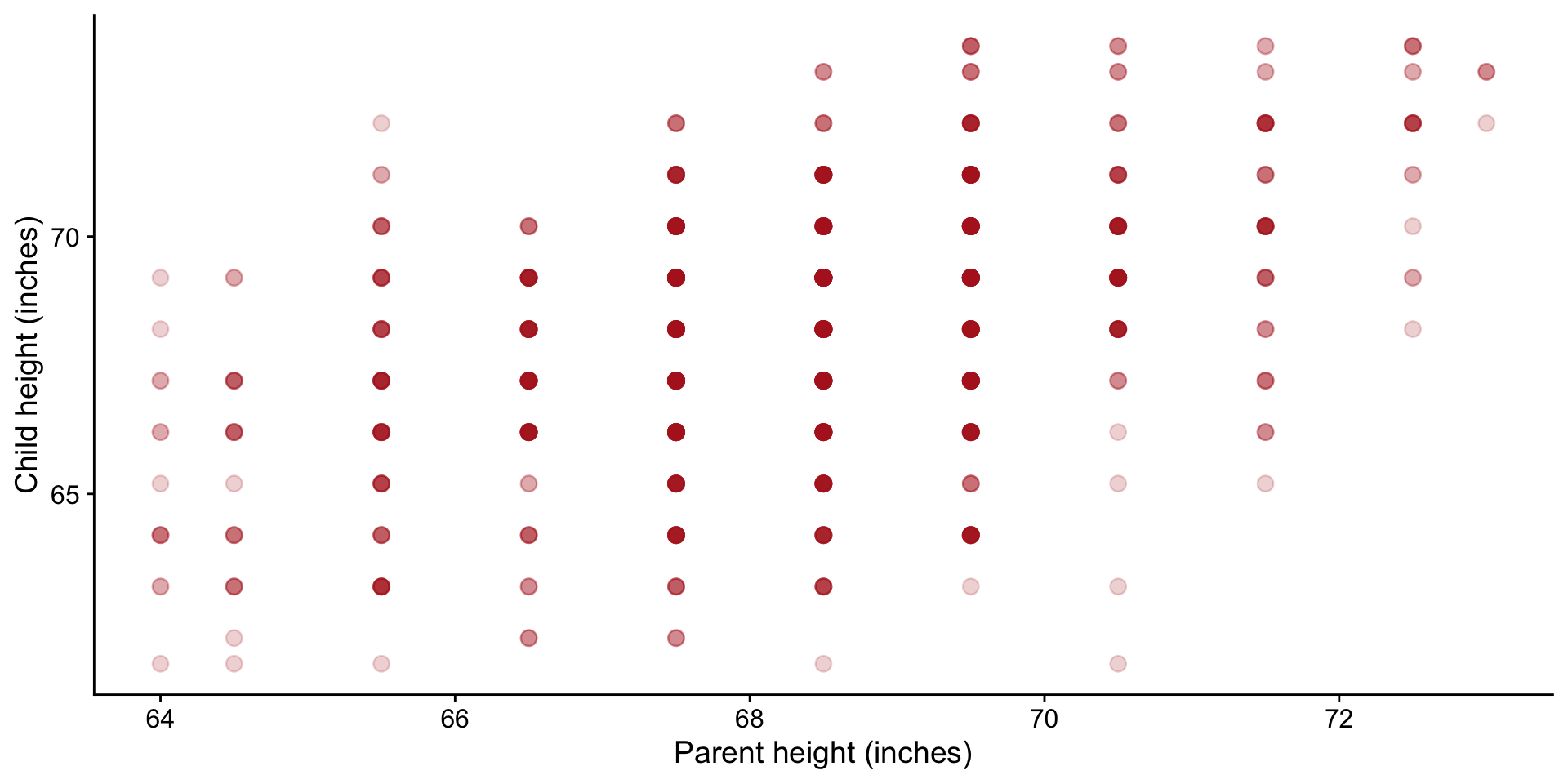
  • 928 children from 205 parent pairs.
  • Parent and child heights were recorded in inches.
  • Heights were recorded in size classes, so the plot will show horizontal bands.

Question: How does child height vary with parent height?

Scatterplot

Scatterplot of child height against parent height, showing a positive but noisy relationship.

We want to explain this noisy relationship…

Regression line

We want to explain this noisy relationship… using a linear model…?

How does linear modelling work?

Least squares

The method of least squares is the automobile of modern statistical analysis: despite its limitations, occasional accidents and incidental pollution, it and its numerous variations, extensions, and related conveyances carry the bulk of statistical analyses, and are known and valued by nearly all.

– Stigler, 1981 (emphasis added)

Residuals, \(\widehat{\epsilon}\)

\[Residual = observed − predicted\] \[ \color{royalblue}{\widehat{\epsilon}_i} = \color{firebrick}{y_i} - \color{forestgreen}{\widehat{y}_i} \]

If a child is 178 cm tall and the fitted line predicts 174 cm, the residual is +4 cm.
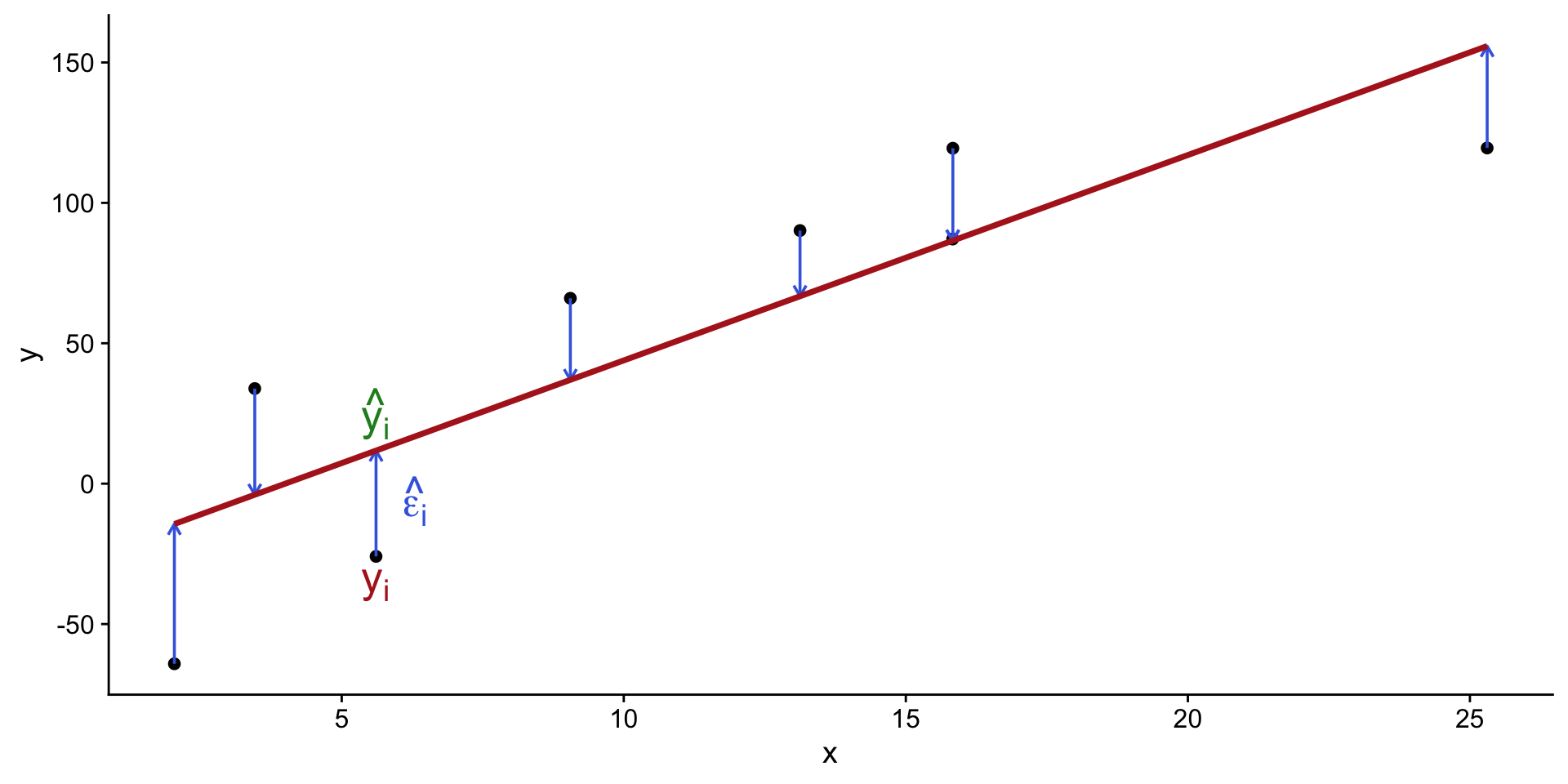
Plot showing observations, a fitted line, and vertical residual distances from each observation to the line.

Using residuals to find the best line

Choose the intercept (\(\beta_0\)) and slope (\(\beta_1\)) that make the total squared residual as small as possible:
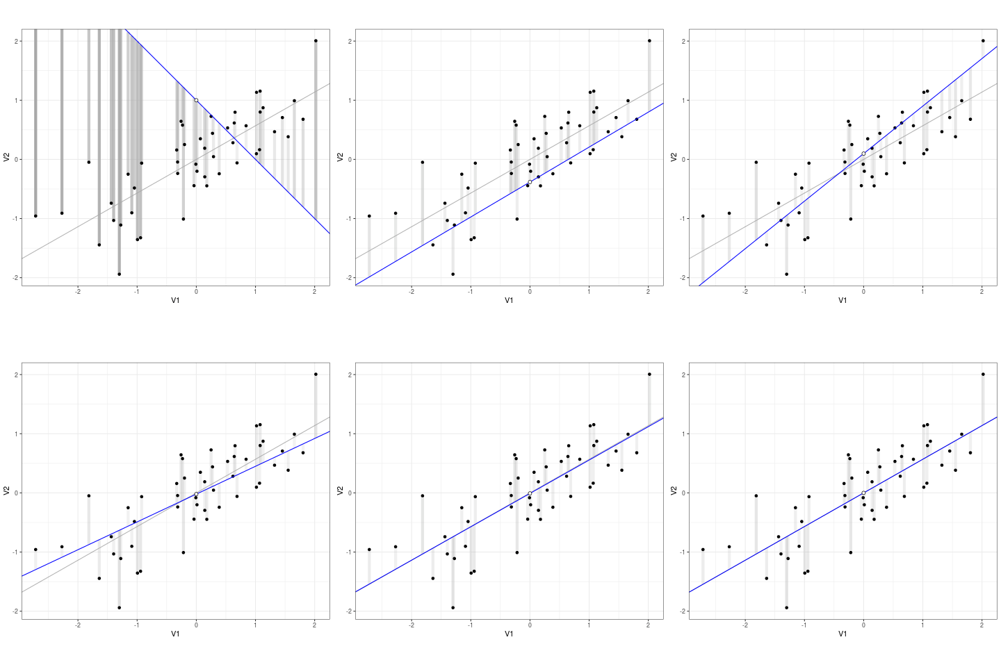
Source: ls-springs

\[\color{firebrick}{\mathop{\mathrm{arg\,min}}_{\beta_0, \beta_1}} \sum_{i=1}^n (y_i - \color{royalblue}{(\beta_0 + \beta_1 x_i)})^2\]

  1. Draw a candidate line.
  2. Calculate the residuals.
  3. Square and sum them.
  4. Find the line with the smallest sum.
  5. Report its slope and intercept.

The linear regression

Model definition

A linear model describes the relationship between a response \(y\) and a predictor \(x\).

\[y_i = \beta_0 + \beta_1 x_i + \epsilon_i\]

  • \(\beta_0\): intercept
  • \(\beta_1\): slope
  • \(\epsilon_i\): deviation of observation \(i\) from the mean response predicted at \(x_i\)

Understanding the model

In the model:

\[y_i = \color{royalblue}{\beta_0 + \beta_1 x_i} + \color{red}{\epsilon_i}\]

The blue component is the fixed mean relationship. The red component is random variation around it.

We can think of the response as being made up of two components:

  • Response = Prediction + Error
  • Response = Signal + Noise
  • Response = Deterministic + Random
  • Response = Explainable + Everything else

How do we “explain” a fitted model?

\[y_i = \color{royalblue}{\beta_0 + \beta_1 x_i} + \color{red}{\epsilon_i}\]

If we were to use plain English, we could say:

The response variable \(y\) changes by \(\beta_1\) units for every 1-unit change in the predictor \(x\), and the average value of \(y\) when \(x = 0\) is \(\beta_0\). The remaining variation in \(y\) is due to random error.

From model to fitted equation

The model:

\[y_i = \beta_0 + \beta_1 x_i + \epsilon_i\]

After fitting the data:

\[\widehat{y}_i = \widehat{\beta}_0 + \widehat{\beta}_1 x_i\]

For Galton’s data:

\[\widehat{child} = 23.94 + 0.65(parent)\]

Once we fit the model, it is now called an estimate (although other terms are also used, such as “fitted value” or “predicted value”), and we no longer have the error term because we are now describing the mean response at each value of \(x\).

Interpretation?

\[\widehat{child} = 23.94 + 0.65(parent)\]

Term Estimate (SE) 95% CI p-value
Coefficients
Intercept 23.94 (2.81) 18.43–29.46 <0.001
Parent height (in) 0.65 (0.041) 0.57–0.73 <0.001
Model fit
0.21
Adjusted R² 0.21
n 928
SE = standard error; CI = confidence interval.

\[\widehat{child} = 23.94 + 0.65(parent)\]

Term Estimate (SE) 95% CI p-value
Coefficients
Intercept 23.94 (2.81) 18.43–29.46 <0.001
Parent height (in) 0.65 (0.041) 0.57–0.73 <0.001
Model fit
0.21
Adjusted R² 0.21
n 928
SE = standard error; CI = confidence interval.

A 1-inch increase in parent height corresponds to a 0.65-inch increase in predicted mean child height. This value corresponds to \(\widehat{\beta}_1\), the estimated slope of the fitted line.

\[\widehat{child} = 23.94 + 0.65(parent)\]

Term Estimate (SE) 95% CI p-value
Coefficients
Intercept 23.94 (2.81) 18.43–29.46 <0.001
Parent height (in) 0.65 (0.041) 0.57–0.73 <0.001
Model fit
0.21
Adjusted R² 0.21
n 928
SE = standard error; CI = confidence interval.
  • If you see SE, that’s the standard error of the estimated slope. It describes how precise the estimate is.
  • If you see a 95% CI, that indicates the range of slope values we are confident that if we repeated the experiment many times, 95% of the time the true slope would fall within that range.
  • The \(p\)-value tests the null hypothesis that the slope is zero. A small \(p\)-value indicates that the slope is unlikely to be zero, and we can conclude that there is a significant linear association between parent and child height.

\[\widehat{child} = 23.94 + 0.65(parent)\]

Term Estimate (SE) 95% CI p-value
Coefficients
Intercept 23.94 (2.81) 18.43–29.46 <0.001
Parent height (in) 0.65 (0.041) 0.57–0.73 <0.001
Model fit
0.21
Adjusted R² 0.21
n 928
SE = standard error; CI = confidence interval.

The intercept is \(\widehat{\beta}_0\), the estimated mean child height when parent height is zero. Does this make sense?

\[\widehat{child} = 23.94 + 0.65(parent)\]

Term Estimate (SE) 95% CI p-value
Coefficients
Intercept 23.94 (2.81) 18.43–29.46 <0.001
Parent height (in) 0.65 (0.041) 0.57–0.73 <0.001
Model fit
0.21
Adjusted R² 0.21
n 928
SE = standard error; CI = confidence interval.

\(R^2 = 0.21\) explains that parent height accounts for 21% of the observed variation in child height. Adjusted \(R^2\) applies a penalty for model complexity. With one predictor and 928 observations, it remains 0.21. Finally, \(n\) is the number of observations used to fit the model.

Putting the result into words

\[\widehat{child} = 23.94 + 0.65(parent)\]

  1. Statistical interpretaion
  2. Biological interpretation

There was a significant, positive linear association between parent and child height (95% CI 0.57–0.73, p < 0.001), and the model accounted for 21% of the variation in child height. A 1-inch increase in parent height corresponded to a 0.65-inch increase in predicted mean child height.

Practice

Example: Adelie penguins

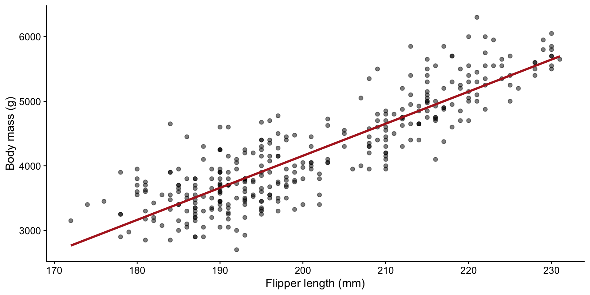
lm(formula = body_mass_g ~ flipper_length_mm, data = penguins)

Residuals:
    Min      1Q  Median      3Q     Max
-875.68 -331.10  -14.53  265.74 1144.81

Coefficients:
                   Estimate Std. Error t value Pr(>|t|)
(Intercept)       -2535.837    964.798  -2.628  0.00948 **
flipper_length_mm    32.832      5.076   6.468 1.34e-09 ***
---
Signif. codes:  0 '***' 0.001 '**' 0.01 '*' 0.05 '.' 0.1 ' ' 1

Residual standard error: 406.6 on 149 degrees of freedom
  (1 observation deleted due to missingness)
Multiple R-squared:  0.2192,    Adjusted R-squared:  0.214
F-statistic: 41.83 on 1 and 149 DF,  p-value: 1.343e-09

Example: Iris setosa

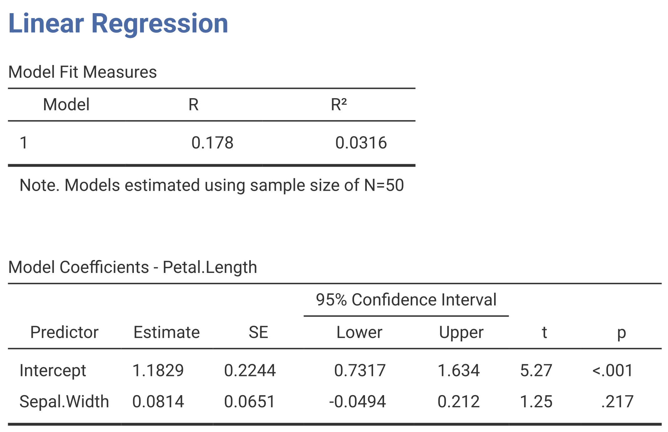
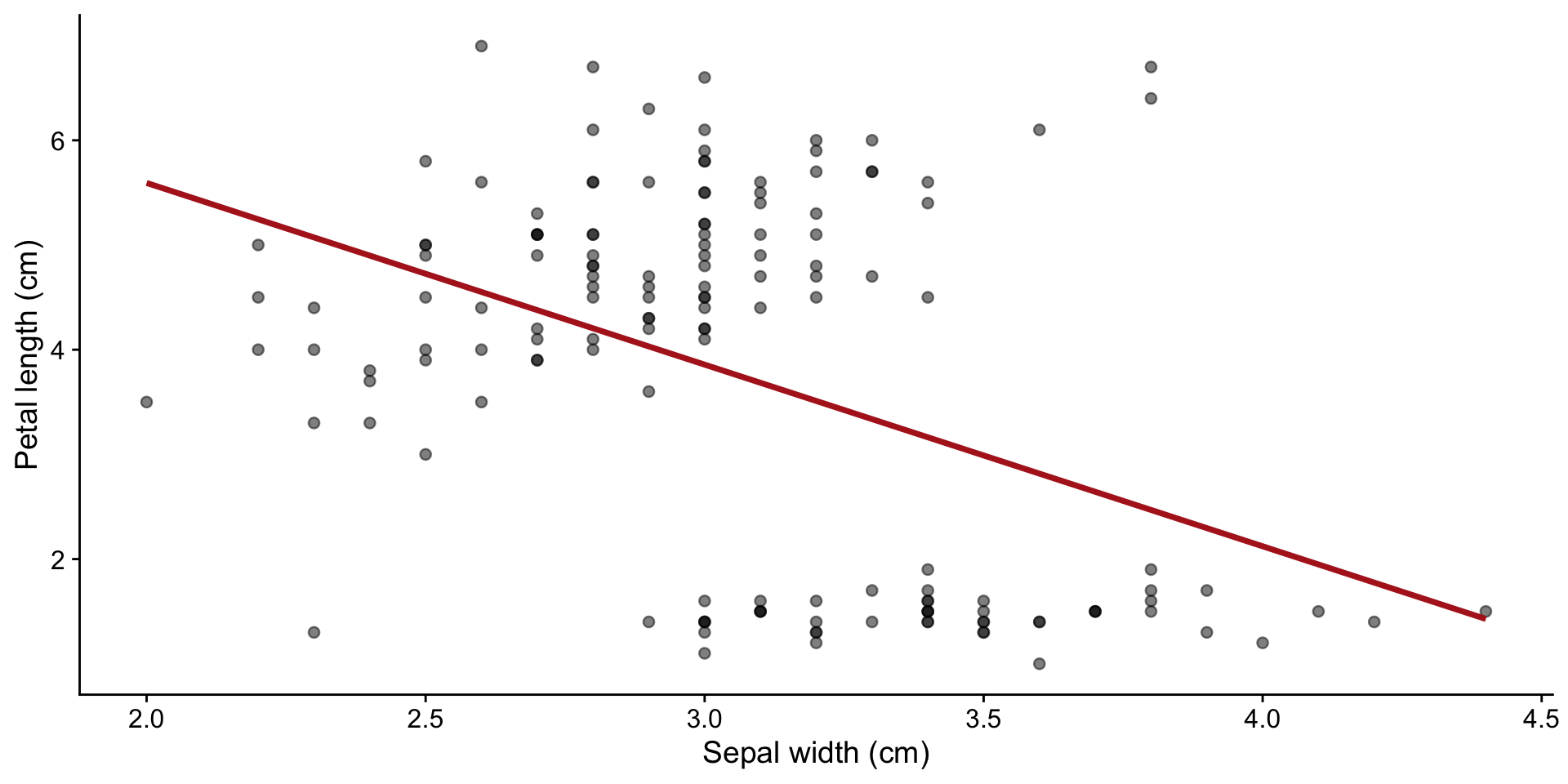
Jamovi linear regression output for petal length predicted by sepal width in 50 Iris setosa observations.

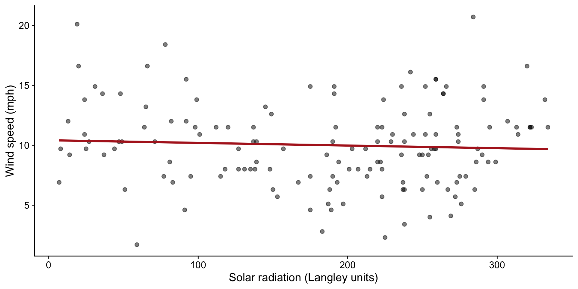
Example: Air quality data

Code
# Remove missing values and fit linear model
air_clean <- airquality |> filter(!is.na(Solar.R), !is.na(Wind))
fit_air <- lm(Wind ~ Solar.R, data = air_clean)

air_summary <- summary(fit_air)
air_coefficients <- air_summary$coefficients
air_confidence <- confint(fit_air)

tibble(
  term = c("Intercept", "Solar radiation (Langley units)"),
  estimate_se = sprintf(
    "%.3f (%.3f)",
    air_coefficients[, "Estimate"],
    air_coefficients[, "Std. Error"]
  ),
  ci = sprintf("%.3f to %.3f", air_confidence[, 1], air_confidence[, 2]),
  p = format.pval(air_coefficients[, "Pr(>|t|)"], digits = 2, eps = 0.001)
) |>
  gt() |>
  cols_label(
    term = "Term",
    estimate_se = "Estimate (SE)",
    ci = "95% CI",
    p = "p-value"
  ) |>
  cols_align(align = "right", columns = c(estimate_se, ci, p)) |>
  tab_source_note(
    source_note = sprintf(
      "Model fit: R² = %.3f; adjusted R² = %.3f; n = %d.",
      air_summary$r.squared,
      air_summary$adj.r.squared,
      nobs(fit_air)
    )
  ) |>
  style_results_table()
Term Estimate (SE) 95% CI p-value
Intercept 10.415 (0.669) 9.092 to 11.738 <0.001
Solar radiation (Langley units) -0.002 (0.003) -0.009 to 0.004 0.5
Model fit: R² = 0.003; adjusted R² = -0.004; n = 146.

A fitted model is not automatically a good model

Any dataset can be given a fitted straight line, but that does not mean the line describes the data well.
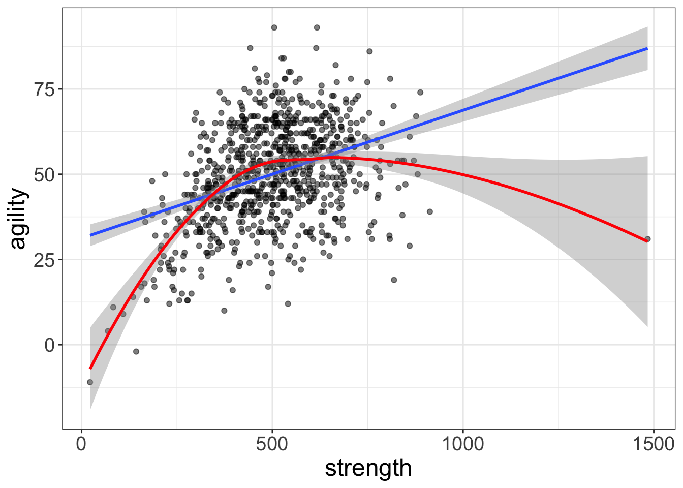
Two models fitted to the same data.

Next week: model assumptions

We will explore the assumptions of linear regression and learn how to assess whether they are reasonable for our data.

Thanks

This presentation is based on the SOLES Quarto reveal.js template and is licensed under a Creative Commons Attribution 4.0 International License.